Dynamics 365FO/AX Finance & Controlling

Parallel inventory valuation – an alternative approach (Part 5)

As the other remaining production related standard cost variances are treated in a similar way as the previously analyzed lot size variance, they are analyzed together in this post. In order to get a price, quantity and substitution variance posted, the following modifications have been made to the standard production process for the item that has already been used in the prior post.

1. Instead of consuming one raw material, two pieces of the raw material are consumed, which results in a quantity variance of $500.
2. The standard cost price of the raw material has been increased from $500 to $515 prior to the start of the production order. This gave rise to a price variance of
   2 pcs x ($515-$500) = $30
3. The route card was posted with a different route version, which had a different (more expensive) cost category price setup ($600 instead of $490). This change resulted in a substitution variance of $110.

 Other common sources of standard cost variances are described on the following website: https://technet.microsoft.com/en-us/library/gg213654.aspx

The next screen print illustrates the total production costs of $1640 and the different standard cost variances for the sample production order processed.

As before, the next accounting overview summarizes the generated ledger transactions.

The grey highlighted lines offset each other and can thus be ignored for the analysis of the production costs.

For those readers who are not very familiar with ledger postings, the following financial statement overview has been prepared.

The financial statement overview presented above shows that the total inventory balance of the produced item ($1000) is too low from an actual costing perspective ($1640). For that reason, an allocation of the price, quantity and substitution variance similar to what has been shown in the previous post for the lot size variance is required.

Applied to the example shown above, the complete price, quantity and substitution variance amounts would have to be shifted to the company’s balance sheet by making use of an allocation rule. That is because only a single receipt transaction but not issue transaction has been recorded thus far. If also issue transactions would have been recorded, a separation and allocation of the different variance amounts would be required. The setup and application of this allocation rule is not shown here to conserve space and because it follows the same concept that has been explained in the prior posts.

Summary:This and the previous posts demonstrated that companies that make use of a standard cost inventory valuation can obtain a parallel inventory value that is based on actual costs by applying general ledger allocation rules for the different standard cost variances.

The next graph summarizes the different standard cost variances and illustrates how they need to be treated to arrive at a parallel inventory value.

The graph above differentiates between the different standard cost variances based on whether they arise internally (cost revaluation and cost change variance) or whether they have an external market relationship.

External market relationship in this context refers to the purchase market, which gives raise to the purchase price variance in case items are purchased and to the sales market, which relates to the produced items once they are sold.

As explained before, the ‘internal’ standard cost variances need to be eliminated, that is, shifted from the company’s income statement to its balance sheet because they relate to receipt transactions only and are eliminated automatically once the items are sold/consumed later on.

The ‘external’ standard cost variances require on the other hand side a separation based on whether they relate to receipt or issue transactions. This separation can be realized by making use of the ledger allocation rules and ensures that an actual cost inventory value can be obtained.

Overall it can be concluded that a parallel inventory valuation can be realized for companies that make use of standard costs by applying general ledger allocation rules. This post concludes this series on the alternative parallel inventory valuation approach. I hope that you found the one or the other useful information. Till next time.

Parallel inventory valuation – an alternative approach (Part 4)

After the purchase and internal standard cost variances have been analyzed, let’s now have a look at the production related standard cost variances and how to deal with them.

Within this fourth part we will have a look at the lot size variance (LSV) first, which arises for example if the good quantity from a production order differs from the calculation quantity that was used for the standard cost calculation of an item. The following graphic illustrates the composition of the finished item that will be used for the subsequent explanations of the production lot size variance.

The graphic above shows a finished good that is made of a raw material that has a standard cost price of $500 setup. In addition, another $500 route related costs – that consist of $490 assembly cost and $10 setup cost – are necessary to produce the item.

As the setup costs are independent from the quantity produced, the total production costs of an item decrease, as the production quantity increases. The next graphic illustrates this relationship for the sample item used.

To illustrate how the lot size variance arises and how to deal with this kind of variance, a production order for 10 pcs of the finished good is processed. The next screen print shows that a total of $9910 production costs arise for the production of the 10 items [$10 setup costs + 10 x ($500 material costs + $490 assembly costs)]. The illustrated lot size variance of $90 results from the fix cost degression effect shown in the previous graphic.

Similar to what has been shown in the previous post, the next accounting-like overview summarizes the production postings recorded (separated by the different production steps).

 The grey highlighted lines offset each other and can thus be ignored for the analysis of the production costs.

For those readers who are not very familiar with ledger postings, the following financial statement overview has been prepared.

The financial statement overview shows a total inventory value of $10000 for the finished product on ledger account 140670. To produce those finished goods, raw materials with a total value of $5000 and $4910 labor costs have been consumed. The remaining difference to the standard cost value of the finished goods is assigned to the lot size variance that is recorded on ledger account 540630.

Further above, a realized cost amount of $9910 has been identified. Against the background of this actual cost amount, it can be concluded that the inventory value of the finished goods is overstated by $90 from an actual costing perspective.

If one of the produced items is sold later on, the inventory value is decreased by $1000 – the standard costs of the item. The financial statements illustrated below exemplifies this situation.

From an actual costing perspective, the decrease in the inventory value from the sale of the produced item is comparatively too high. The same holds for the cost of sales, which are recorded on ledger account 640650.

In order to arrive at an actual cost valuation, the lot size variance (LSV) needs consequently be adjusted and split up in a similar way that has been shown for the purchase price variance before. The next graphic exemplifies the necessary separation of the total lot size variance if one out of the ten produced items is sold.

To conserve space, the setup of the necessary ledger allocation rule is left as an exercise for the reader. If the allocation rule is later on processed, the following financial statements result:

The financial statement overview shows a total inventory value that is $81 lower than before. This reduction takes care of the difference between the actual and the standard cost price [9 pcs x ($1000 – $991)]. As the allocated lot size variance amount is recorded on a separate ledger account, a parallel standard cost and actual cost inventory valuation can be achieved.

Please note that this also applies for the COGS amount of $1000 that has been adjusted through a corresponding adjustment on ledger account 640651 to arrive at an actual cost value of $991.

Within the next post we will take a look at the other production related standard cost variances and how to deal with them from a parallel valuation perspective. Till then.

Parallel inventory valuation – an alternative approach (Part 3)

The next standard cost variance type that has an influence on the parallel valuation approach concerns cost change variances, which can result from two different sources that will be explained in the following.

Source 1: Standard cost price differences between sitesStandard costs can be setup in a way that different standard cost prices are defined per site in order to incorporate cost price differences resulting for example from transportation costs, etc. The next screen print exemplifies an item that has different cost prices setup for site 1 and site 2.

In order to illustrate what influence these different cost prices have on the parallel inventory valuation approach, 100 pcs of the item have initially been acquired through an inventory adjustment journal for site 1. The resulting financial data can be identified in the following screen print.

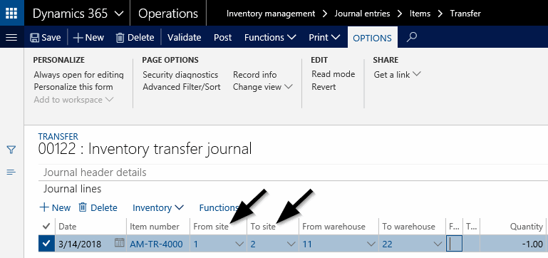
After the items have been acquired, an inventory transfer from site 1 to site 2 for a single item is posted through an inventory transfer journal.

The outcome of this transfer is an adjustment voucher that results in a corresponding increase in the inventory value. The adjustment voucher and the resulting inventory value increase can be identified in the following figures.

What one can identify from the financial statement reports exemplified above is that the total inventory value increased by $25 because of the item transfer from site 1 to site 2.

Before analyzing how to deal with that variance for the parallel inventory valuation approach, let’s have a look at the second possible source of cost change variances.

Source 2: Customer item return after standard cost price change

A second possible source for cost change variances are situations where standard cost items are sold to customers and returned after a cost price adjustment has been completed.

The following example illustrates this scenario where initially 100 pcs of a standard cost item with a cost price of $100/pcs are acquired – for reasons of simplicity – through an inventory adjustment journal. The next screen print shows the resulting financial statements.

After the items have been acquired, 5 pcs are sold for a sales price of $200/pcs. With a standard cost price of $100/pcs, the company’s inventory value is consequently reduced by $500, which can be identified from the next financial statement illustration.

Shortly after the items have been sold, the standard cost price of the remaining inventory items is adjusted from $100 to $130. The resulting accounting voucher and financial statements are shown in the next screen prints.

The screen prints above illustrate that the change in the standard cost price resulted in a $2850 higher inventory value [95 pieces x ($130-$100)].

After the standard cost price has been increased from $100 to $130, the customer decided to return 3 out of the 5 pcs sold. Posting the return order packing slip and invoice results in a number of transaction vouchers that are summarized in the next accounting-like overview.

 The grey highlighted lines offset each other and can thus be ignored for the analysis of the production costs.

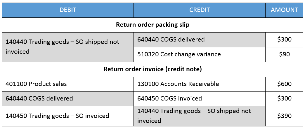
The transaction vouchers summarized above demonstrate that the item return resulted in a corresponding adjustment of the sales revenue and the receivables amount (3 pcs x $200 sales price / pcs = $600). At the same time, an adjustment of the COGS and inventory value was recorded. Yet, because of the cost price change, a $90 higher inventory value remains.

Expressed differently, selling and returning the 3 items resulted in a $90 higher inventory value, which can be identified in the following financial statement overview.

After having analyzed the sources of cost change variances, the question arises, how to deal with them in order to arrive at a parallel actual cost based inventory value? 

As mentioned in the previous post, standard cost price changes resp. differences typically do not reflect actual (market) price differences but rather cost/transportation/handling cost differences.

Moreover, in an actual inventory costing environment, internal movements of goods between different sites do not affect the company’s profit. That is, a company does not get richer or poorer by the mere fact that an item has been shifted from one location to the other, as it might be the case for standard cost items.

The same holds for the second source of the identified cost price changes; i.e. in an actual costing environment, a company does not get richer or poorer by shipping and returning goods to and from a customer, as it might be the case in a standard cost environment.

For those reasons and because cost change variances affect receipt transactions only, it can be argued that the complete cost change variance amount needs to be shifted from the company’s income statement to it’s balance sheet in order to arrive at an approximate actual cost valuation. This shifting can once again be realized by making use on an allocation rule similar to the one that has been introduced in the prior posts.

The next posts will deal with the production related standard cost variances and how to incorporate them in the parallel inventory valuation approach. Till then.

Parallel inventory valuation – an alternative approach (Part 2)

After having analyzed how to deal with purchase price variances in order to arrive at a second (parallel) inventory value, let’s have a look at the second standard cost variance type – the inventory cost revaluation – and how to deal with those variances to obtain a second (parallel) inventory value for standard cost items.

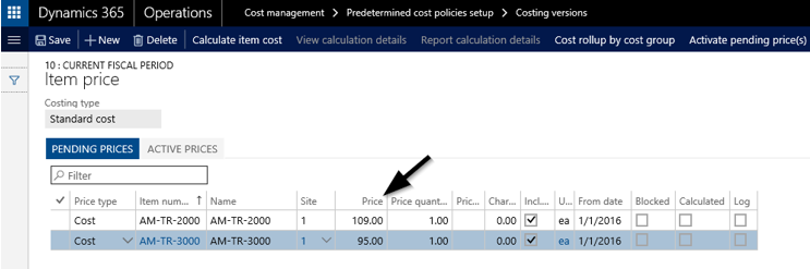
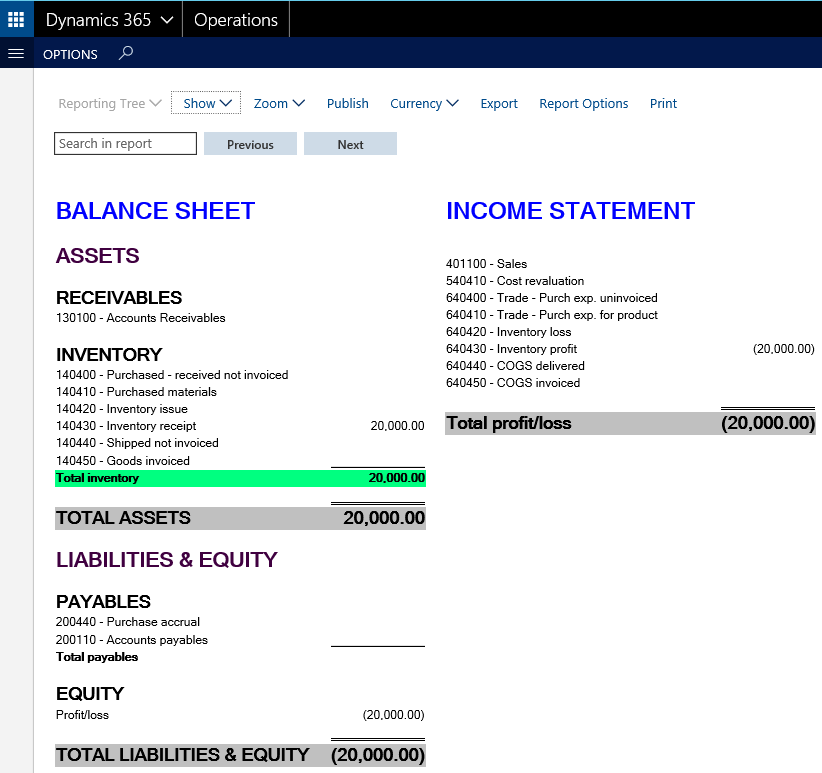
Scenario:At the end of a fiscal year, the standard costs of a first item are adjusted from $100 to $109. For a second standard cost item, the standard costs are adjusted from $100 to $95. As there are currently 100 pcs from each of the items on stock, a total inventory value of $20000 can be identified (before adjusting the standard cost prices) in the financial statements illustrated in the next figure.

 For reasons of simplicity the inventory values/balances have been created by posting an inventory adjustment journal that resulted in an inventory receipt & profit transaction.

The aforementioned revaluation of the standard cost item is realized by recording and activating the new standard cost prices in the standard cost costing version, as exemplified in the next screen print.

Once the new standard cost prices are activated, the financial statements show a $400 higher inventory value. This can be identified from the next figure.

The overall increase in the inventory value can be explained by the value increase of the first standard cost item [($109-$100) x 100 pcs] and the value decrease of the second standard cost item [($95-$100) x 100 pcs]. If the revalued items will be sold subsequently, the newly activated standard cost prices will be used for posting the issue transactions.

At this point the question arises whether the inventory cost revaluation amount can remain in the income statement as illustrated in the previous screen print or whether an adjustment similar to the one that has been shown in the first part for the purchase price variance (PPV) is required in order to get a second (parallel) inventory value?

This question can be answered by stating that no split and allocation of the cost revaluation is required, if the cost revaluation is done in a way to adjust the standard cost prices to an ‘actual’ market price. If this is the case, any previously recorded adjustment and allocation of the PPV needs to be reversed in order to avoid an over-adjustment of inventory values towards actual market prices/values.

In practice, most companies do not adjust their standard cost prices in a way to reflect ‘actual’ (market) cost prices. Otherwise, they would have chosen an alternative actual cost price valuation model right from the beginning. Against the background of this common adjustment behavior, it can be argued that an adjustment of the recorded standard cost revaluation amount is necessary in order to arrive at an approximated actual inventory cost price. The main question in this context is then how such an adjustment can be realized?

From the authors’ perspective, the complete cost revaluation amount needs to be shifted (allocated) from the income statement to the balance sheet in order to arrive at an actual cost valuation amount. That is because only those items that are currently on stock (or in process) – that is receipt transactions – are affected by the cost change variance. If those items are sold or consumed later on the adjusted higher/lower standard cost price will ensure that the cost revaluation amount that has been allocated to the balance sheet is successively eliminated. For that reason no split up and allocation of the cost revaluation amount is necessary.

The next part of this series continues with analyzing cost change variances and how they need to be incorporated into this parallel inventory valuation approach.

Parallel inventory valuation – an alternative approach (Part 1)

In one of my prior posts I already had a look at the parallel inventory valuation issue. For details, please see this site.

While the prior post focused on the Russian dual warehouse functionality, this post focuses on an alternative parallel valuation approach I recently came across. A major advantage of this alternative approach compared to the Russian dual warehouse functionality is that it does not depend on country-specific features but rather makes use of generally available functionalities that can be applied in every Dynamics AX/365 for Operations environment.

Let’s get started by having a look at the underlying business scenario for this parallel inventory valuation approach.

Scenario:The following illustrations and explanations are based on a company that makes use of standard costs but requires an ‘actual cost’ evaluation for external reporting & tax purposes.

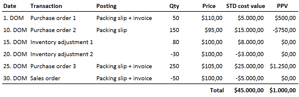
In order to explain the underlying parallel inventory valuation approach, the following sample transactions have been recorded for a trading item; that is, an item which is not used in the production process.

 (DOM = Day Of the Month)

The sample transactions illustrated in the previous figure start with the purchase of 50 pcs of the trading item for a price of $110. As the item is set up with a standard cost price of $100, a purchase price variance (PPV) of $500 results.

The second sample transaction also relates to a purchase order where another 150 pcs of the item are purchased for a price of $95. The major difference between the first and this second transaction is that the second one is only packing slip updated whereas the first one is packing slip and invoice updated.

The third and fourth sample transactions represent (internal) inventory adjustment postings for which no purchase price variance arises.

Those internal transactions are followed by a third purchase order related transaction where another 250 pcs of the item are purchased for a cost price of $105.

Finally, 50 pcs of the trading item are sold to a customer. As the item is set up with standard costs of $100, the inventory value is reduced by a total of $5000.

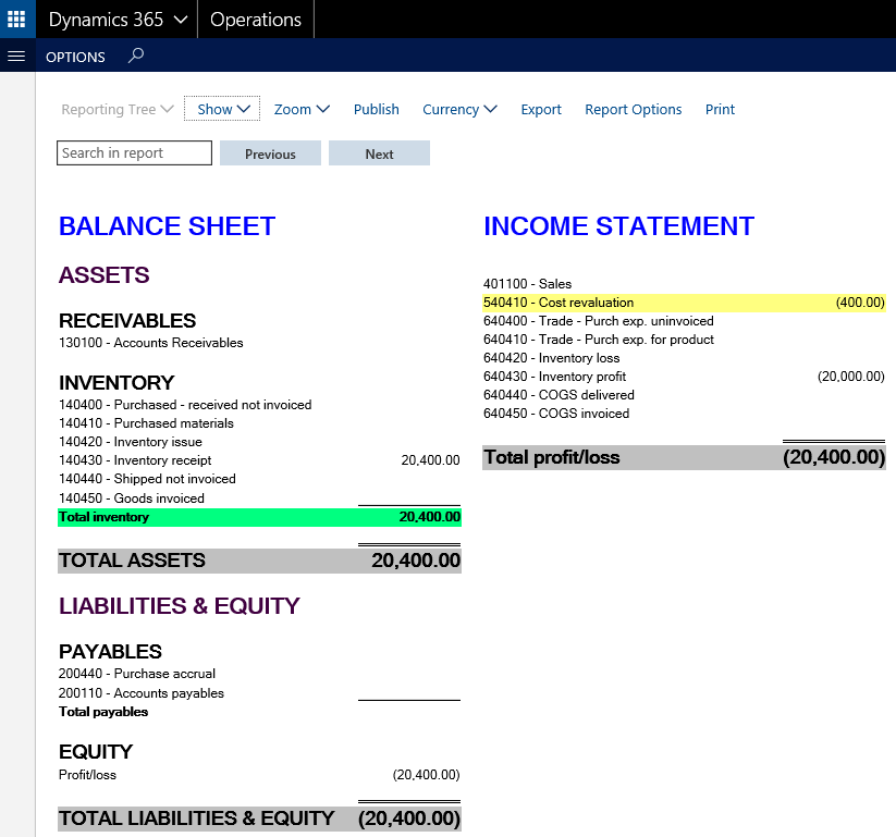
After all sample transactions are recorded, an inventory value of $45000 remains in the balance sheet (BS) and a PPV of $1000 in the income statement (IS). The next figure illustrates the respective financial statement reports.

My next step was making a manual inventory value calculation for the sample transactions in order to get an impression of the theoretically correct actual cost inventory value. To achieve this, an average cost price has been calculated before recording the different (internal and external) issue transactions. This calculation is similar to what one can identify in Dynamics AX for a weighted average cost price valuation and is exemplified in the following figure.

 Depending on how the average values are calculated – before each issue transaction or for the whole period – different actual cost inventory values result. As an example, if a single average cost price is calculated and used for the valuation of the issue transactions, a total inventory value of $45849.06 results. Those valuation differences do, however, not matter here because they have only been shown for explanatory purposes.

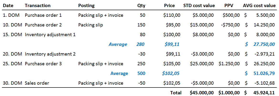
What matters though is the fact that the issue transactions, which have been recorded with the standard cost prices, require some adjustments in order to arrive at an actual cost value. The way how those adjustments can be calculated is illustrated in the following figure.

What can be identified from the previous figure is that the total PPV is split up based on the relationship between the total receipt and total issue transactions. As an example, the $868.85, which are assigned to the total receipt transactions are calculated as follows: $1000 / ($53000 + $8000) * $53000.

 If only external receipt and issue transactions are taken into account; that is, if the inventory adjustment transactions, which did not generate a PPV are excluded from the calculation, the following PPV amounts are calculated and can be assigned to the receipt and issue transactions recorded.

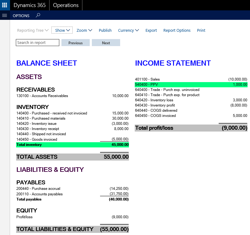
Building upon the last separation of the total PPV, an actual cost inventory value can be approximated by shifting the fraction of the PPV that can be assigned to the receipt transactions from the income statement to the balance sheet. The next illustration exemplifies this.

After having analyzed the theoretical concept how an actual cost inventory value can be approximated for a company that uses standard costs, the question arises how this theoretical concept can be implemented into Dynamics AX/365 for Operations?

The answer to this question are General Ledger (GL) allocation rules that can be used for transferring the part of the PPV, which relates to the receipt transactions, into the company’s balance sheet.

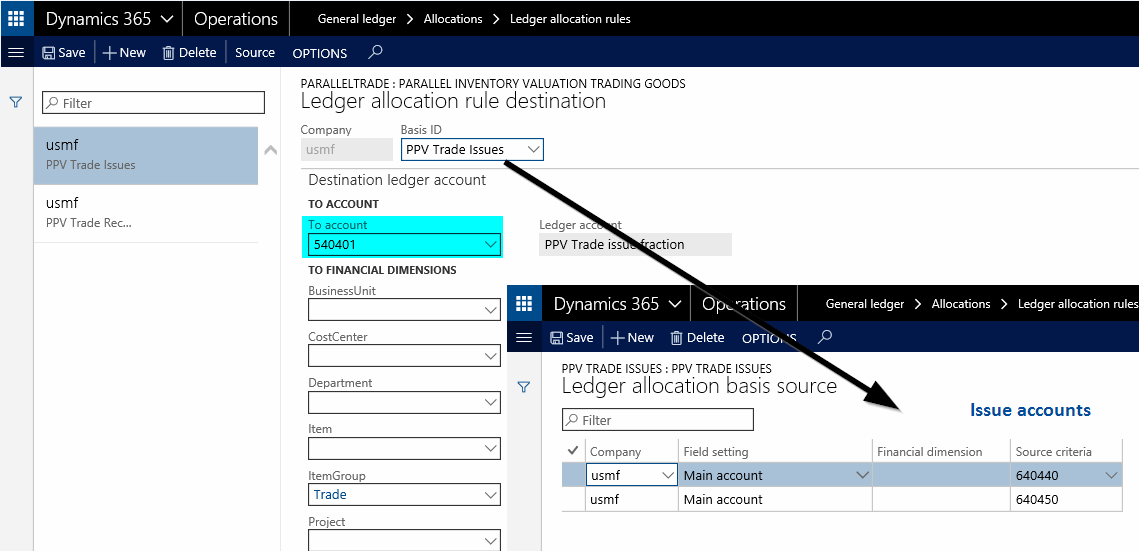
The next screen print shows the allocation rule used. Please note that this rule is set up with the ‘basis’ allocation method.

The ledger account that records the PPV for the trading items – account no. 540400 in the example – is included in the ledger allocation source form and will be used as the basis for the subsequent allocation calculation.

 Please note that the allocation basis is defined in combination with the financial dimension ‘item group’, which has been assigned to all trading items. Referring to the item group rather than using separate allocation rules for each individual trading item is a simplification that will not result in an individual but a group-based inventory valuation of the item. From the author’s perspective, this simplification appears to be justifiable, as companies regularly do not report inventory values on an individual item basis in their external financial statements.

The next setup required for using ledger allocation rules concerns the offset account, which should be different from the PPV account that is used in the ledger allocation source form shown above in order to allow users tracking the original and adjusted PPV.

Finally, ledger allocation rule destinations have to be set up that define the account-financial dimension combinations to which the PPV will be allocated.

The next screen prints show that the part of the PPV that relates to the issue transactions is recorded on the income statement account 540401. The part of the PPV that relates to the receipt transactions is, on the other hand side, recorded on the balance sheet account 140499.

 

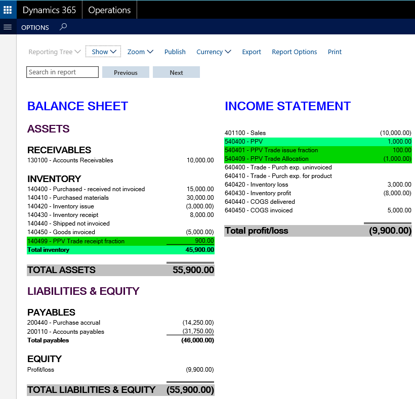
Once the ledger allocation rule is setup and activated, it can be processed. Processing the exemplified allocation rule results in the following voucher, which debits the PPV income statement account 540401 for the part of the PPV that remains in the income statement. The remainder of the PPV is consequently shifted to the balance sheet account 140499. In order to avoid a double counting of the PPV, the credit transactions on the income statement account 540409 offsets the posted PPV.

The following screen print summarizes the resulting balance sheet and income statement reports after the allocation rule is processed and posted.

Assessment:The parallel inventory valuation approach illustrated in this post requires that all items are set up with an ‘item group’ or ‘item’ financial dimension. In addition, separate issue and receipt accounts need to be set up for the different inventory transaction types.

Apart from those setup considerations, major disadvantages of the approach demonstrated here comprise:

1. That the ‘actual’ inventory cost value can be identified at the General Ledger level only, and
2. That the approach illustrated requires the use of standard costs.

Despite those disadvantages, the inventory valuation approach demonstrated here seems to be much better suited than alternative approaches the author came across, such as creating specialized and complex inventory transactions reports that are used for recording manual adjustment postings at the General Ledger level or doing some ‘creative’ Excel calculations in order to arrive at an actual cost value amount which is subsequently posted in the system. What is more, the approach illustrated here is in line with the ‘specific identification’ valuation methods that are allowed to be used by IFRS and US-GAAP.

The next post will extend the approach exemplified here to the other standard cost price variances. Till then.